Modeling Architectural Microclimate Effects: Which Approach, When?

A model is a representation — typically simplified and/or idealized — of a ‘thing’ (e.g., a structure, a system, a phenomenon, etc.). In scientific pursuits, wind models are used to help explore, examine, and explain, ultimately increasing our understanding of how the ‘thing’ represented by the model works and interacts with its surroundings.

In architectural engineering, models play a vital role in the design process. Wind engineers rely on modeling to understand how a building impacts, and is impacted by, its surroundings. For example, models can predict local microclimate effects like airflow patterns, which are combined with wind comfort and safety criteria to perform Pedestrian Level Wind (PLW) analysis.

Until recently, only a couple of wind modeling options have been available — but new methods are emerging. While more options are generally a good thing, more choice can also lead to confusion about what methods are most appropriate.

In this post, we’ll examine a handful of modeling approaches that can be used to explore wind effects, with the two related goals of:

1. Helping readers to better understand the different approaches available today, including how each works and relative pros and cons; and
2. Determining which approach(es) align with different phases of the architectural design process.

All models are wrong

In their book Empirical Model-Building and Response Surfaces, statistician George E. P. Box and co-author N. R. Draper wrote, “Remember that all models are wrong; the practical question is how wrong do they have to be to not be useful.”

(this advice is likely the source of the ‘quotation’ with which Box is arguably most associated, that “All models are wrong, but some are useful.”)

Because models are representations, as opposed to reproductions, “all models are wrong” is true in a literal (and pedantic) sense. This summary, however, misses the real point of Box and Draper’s original quote: how imperfect must a model be such that it is no longer useful as an aid? How much error can we accept within a model when using it to increase our understanding of the thing it represents?

Appreciating these real-world tradeoffs is essential if we are to make informed decisions. It is in this spirit that we now turn our attention to different microclimate modeling techniques.

Different approaches for modeling microclimate wind effects

Let’s state our goal as wanting to understand PLW around a proposed structure, as a result of that structure’s effect on the local microclimate, as determined by how the structure and surrounding building’s massing interacts with the atmospheric boundary layer (ABL).

To analyze PLW, we need to examine how wind behaves around the structure, and then combine these findings with PLW criteria. In the context of this post, we’ll focus on the first part: understanding wind flows.

Importantly, each of the techniques examined below uses modeling — sometimes physical, sometimes digital/mathematical. Choosing what approach to use depends upon what level of accuracy you’re trying to achieve. It also depends on how much you’re willing to spend —in time, effort, and (of course) currency — to achieve it.

Physical models: ABL wind tunnel tests

Done correctly, testing a structure in an ABL tunnel replicates all of the intricacies of wind flow. This is why such tests are the gold standard when it comes to outdoor flow simulation. For this reason, many zoning boards and other approval bodies rely upon (and often require) such tests to be conducted.

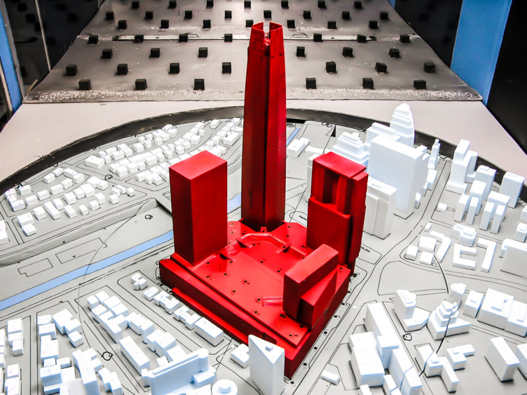
Wind tunnel tests are conceptually very straightforward:

1. Create a miniature a physical model of a structure
2. Place it in a wind tunnel
3. Blast air at the model
4. Measure/observe

But in reality, things are a little bit more complicated than that, for at least a few reasons.

Why wind tunnel testing is so complicated

First, testing architectural structures requires an ABL wind tunnel, which is different from the types of tunnels used to test airfoils, jet engines, and the like. An ABL tunnel conditions upstream wind to approximate a variety of ABL types. It does this by altering the characteristics of the wind flow via elements such as spires and ground roughness blocks.

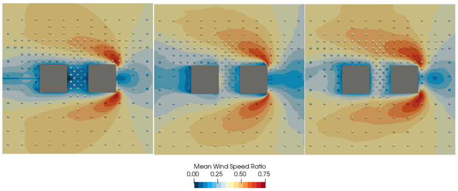
Second, to provide comprehensive analysis, the model has to be rotated to account for different wind directions (often up to 36). This means steps 3 and 4 in the simplified procedure above must be repeated dozens of times.

(It’s worth noting that wind engineers are often more concerned with the combined wind results, not the individual directional ones. The directional results give excellent insight into potentially what is causing challenging conditions. Even so, they are generally not used to determine PLW comfort on their own.

Third, the results depend heavily on Reynolds number scaling, sensor placement (ABL tunnels use a variety of sensor types to measure the air flow at different points around the model), and sensor accuracy: model inaccuracies and sensor issues impact the results. For example, Irwin Probes are highly versatile and are excellent at capturing high speed areas. They are, however, less accurate in wake zones and confined locations (e.g., areas with overhangs where high turbulence levels can occur).

An important practical limitation is that there aren’t very many ABL wind tunnels in existence. This in turn leads to high testing costs and extended testing timelines.

Computational Methods: RANS and LES

Computational fluid dynamics (CFD) uses numerical analysis to examine fluid (in this case, air) flows. Within the broad CFD domain, two approaches are regularly used to model wind effects:

• Reynolds-averaged Navier–Stokes (RANS)
• Large eddy simulation (LES)

The math is made all the more complex because we’re applying numerical analysis to bluff body aerodynamics. This means we have high Reynolds numbers (i.e., inertial forces dominate viscous forces) and full turbulence (i.e., momentum transfer is attributable virtually entirely to random eddies).

In particular, turbulence makes things especially challenging. Without getting super into the details, here are the main ways in which these two approaches differ:

• RANS treats turbulence as a combination of a time-averaged signal plus a fluctuating quantity. This makes it easier to solve the equations but causes transient values to disappear. This approach relies on the assumption that turbulence generally has less kinetic energy than the mean flow, so can be simplified without losing too much accuracy.
• LES solves for transient flows in the time domain, focusing on the big energy structures and applying a simplified approach to high-frequency/low-energy flows that have comparatively little influence on wind effects. By doing so, LES effectively removes small-scale information from the numerical solution, thereby simplifying the calculations and reducing the computational cost.

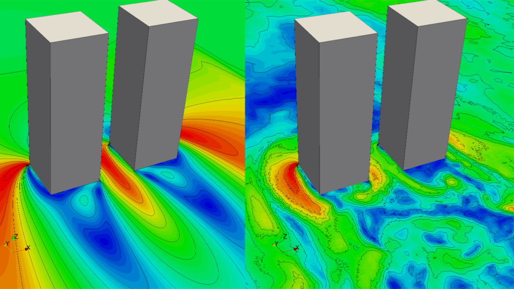
Putting RANS and LES to the test

To assess the capabilities of RANS and LES, RWDI has performed extensive analysis to compare the results of RANS (500+ simulations) and LES (100+ simulations) modeling against tests conducted in RWDI’s state-of-the-art ABL wind tunnel.

The results allow us to understand and quantify the performance of both RANS and LES over a wide spectrum of use cases and configurations. Broadly, the analysis leads to a number of important conclusions:

• In practice, RANS needs to be heavily modified for it to perform adequately for architectural use cases. Using a RANS solver in its out-of-the-box configuration can lead an architecture firm to come to erroneous conclusions. Modifying the solver to improve accuracy requires time, effort, and a highly specialized skillset.
• Even in the best case, RANS tends to perform poorly in deep wake regions (although it does relatively well in accelerated zones).
• LES most closely matches the results of wind tunnel testing; or, in layperson terms, LES is a more accurate than RANS in modeling real-world effects. It is, however, a challenging task to run an LES simulation properly.

However, the increased accuracy LES provides comes at a cost. Such analysis tends to be about an order of magnitude (i.e., 10x) more expensive than RANS, making it impractical for rapidly iterative design scenarios.

Combining RANS and LES

The relative strengths and weaknesses of each approach naturally leads to a question: can they be combined to get the best of both techniques, potentially to deliver higher accuracy at lower cost than LES-exclusive analysis?

Again sparing the details, RWDI’s analysis found that combining the two techniques does improve the quality of wind comfort analysis. In this approach — at times employed by Orbital Stack in our own CFD analysis — LES is applied to create high-quality directional results for critical wind directions (per meteorological data), while RANS computation provides directional results for less-critical directions. It should be cautioned, though, that performing such analysis requires considerable expertise and most approval bodies don’t recognize CFD techniques as a substitute for wind tunnel testing

Artificial intelligence: Machine learning (ML)

While it may not be apparent, the two approaches examined so far are both methods of prediction. In the ABL wind tunnel, small-scale models are used to ­predict the behavior of air around a full-scale building; in the CFD examples, math is used to predict (via calculation) airflow behavior.

But there’s another method of prediction that’s gaining traction in a wide range of applications: the form of artificial intelligence (AI) known as machine learning (ML).

Essentially, machine learning works by using validated training data to ‘teach’ an AI (often a convolutional neural network, or CNN) about the relationships between inputs (e.g., massing models and climate data) and outputs (e.g., airflow paths and patterns).

Because Orbital Stack is part of RWDI Ventures, we have access to RWDI’s urban windflow dataset — which is the largest in the world. Leveraging RWDI’s expertise and decades of data from countless wind tunnel tests allowed us to create an industry-first ML-powered wind simulation engine which uses a fraction of the resources of CFD simulations and returns results in a fraction of the time — but the speed and cost savings are achieved at the expense of accuracy.

Answering the practical question: which approach should be used in what circumstances?

It’s now time to circle back to “the practical question” asked by Box and Draper. Given our understanding of the relative merits and drawbacks of the different approaches, which one should we apply, when?

The answer to the question lies in looking at how the needs of architectural designers changes throughout different project phases. In general, as a design progresses from a feasibility assessment to detailed design:

• The number of iterations decreases (i.e., fewer model-impacting tweaks and options are explored), while the turnaround time for each iteration increases (e.g., from minutes to days, weeks, and even months); and
• The cost of errors and corrections dramatically increases, demanding ever-increasing levels of accuracy.

Considerations by design stage

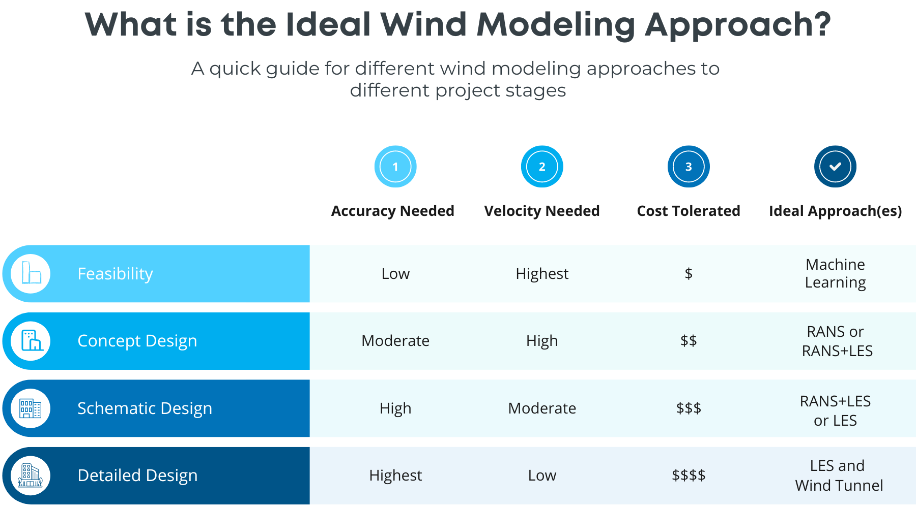
These factors strongly suggest that each of these modeling approaches have an important role to play in the design process:

• Feasibility: The design team explores the feasibility of basic structural shapes and configurations to meet the building’s needs. Quickly reducing the potentials paths forward by learning what won’t work is extremely beneficial, with the intermediate result being one or more initial designs that warrant further exploration. Rapid, low-cost iteration to examine and rule out different design paths is a perfect use case for ML-based modeling.
• Concept Design: The design team needs to be made aware of significant issues with the initial designs that passed the feasibility assessment. At this point, various building massing options are being iteratively explored. This combination of iteration with a need for improved accuracy warrants the use of RANS; more complex designs may also justify augmenting the RANS analysis with LES for particularly important wind directions.
• Schematic Design: The massing is generally decided upon and mostly locked. During this stage, the design team can add smaller elements such as canopies, wind screens and landscaping to improve conditions. Some quantitative feedback is required (e.g., wind speeds are reduced by X% when measure “A” is introduced). Again, a combination of RANS and LES may be appropriate; when greater accuracy is needed for later iterations, designers may transition to LES-only analysis.
• Detailed design: Accurate quantitative results are required, as these are often included in reports that go to local authorities for approval. The design team wants to make sure — and be able to demonstrate to approval bodies — that the design is safe and key areas are fit for purpose (e.g., a café will experience predominantly sitting conditions). In this final design stage, ABL wind tunnel tests or LES studies are most appropriate (and may be required).

Wrapping up

We hope this post has helped you understand the different wind modeling options available today — all have value and utility, but designers should take care to apply the most appropriate modeling technique for each design stage.

If you’re going to ‘go it alone’ with CFD, then please make sure you do so either with the requisite expertise to configure and tune the tools, or with the understanding that out-of-the-box configurations may have severe limitations.

For those who want to skip the effort and headaches associated with tuning and interpreting CFD models, Orbital Stack and RWDI can help:

• Orbital Stack’s ML-powered wind simulation engine is specially designed to enable rapid, low-cost iteration during early design stages.
• Our carefully tuned, purpose-built CFD simulation capabilities leverage RANS and LES to provide more-detailed and more-accurate insights for middle-stage designs.
• RWDI’s renowned wind engineering expertise — including a state-of-the-art ABL wind tunnel — can get even the most complex and groundbreaking designs over the finish line.